Let’s start. Let’s learn about KV Caching, how a simple observation and a rather simple implementation can get you 5x speedup on autoregressive token generation in attention based models. Let’s also implement this using mlx, comparing a naive autoregressive loop implementation against a cached one.

To understand KV Cache, let’s backtrack and understand what are Keys and what are Values, why would be a need to store these values arise, what are the trade offs (there is always a trade off).

I’m assuming who is reading this is familiar with basic attention mechanism and right now let’s only focus on self-attention, also in my implementations later, I will ignore attention masks, position embeddings etc which are necessary for large language models but not so much to demonstrate the use of KV Caching.

Attention Please!

Okay let’s jump right in and let me spoil right away where we are saving computation by trading for a higher memory, the the region of interest for us is where we calculate these Query, Key and Value matrices from input using corresponding weight matrices Wq, Wk, and Wv and to spoil things even more we don’t have to 1) calculate all queries for every new token to predict (only latest is enough) and 2) calculate all keys and value matrices (we can save all previous keys and value matrices, only calculate the latest ones and then save). Now let’s look at some diagrams and later some code in mlx to understand things at a lower level.

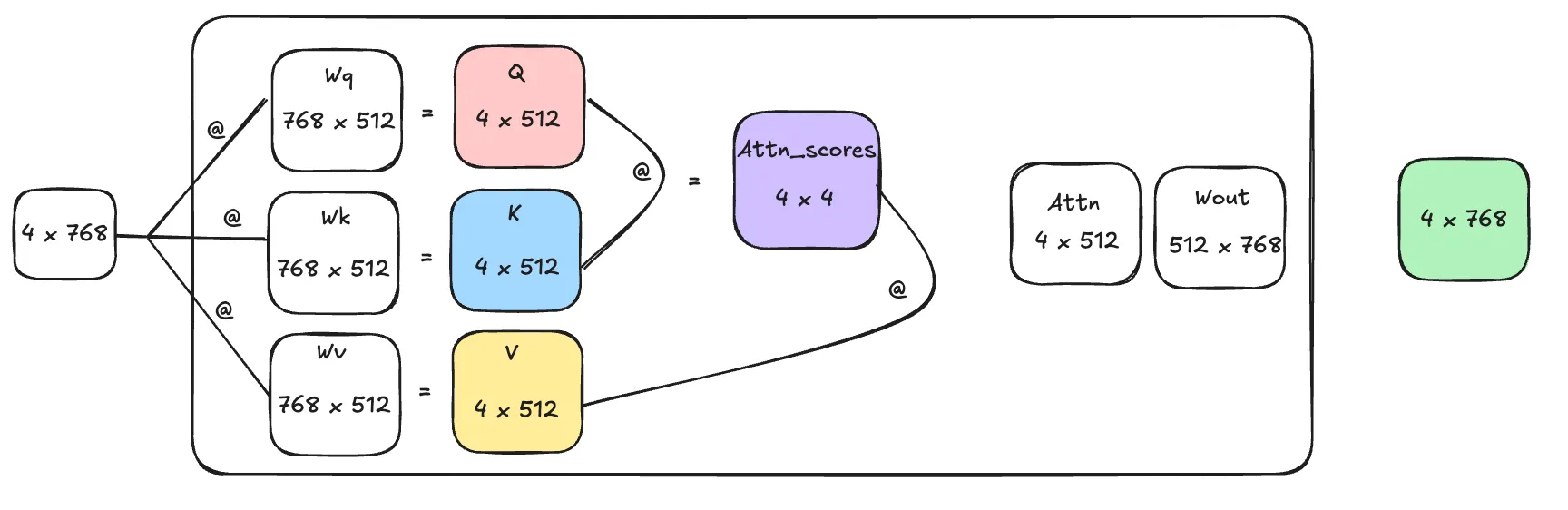
On a high level this is what happens in the attention block. @ denotes matrix multiplication here. We start with a input of dimension 4x768 which is then projected to a different dimension of three different matrices called Query, Key and Values. Queries and Keys are used to calculate attention scores, which contains information about the “relevancy” of each token with respect to another. Then we use these attention scores to modify the Value matrix and using Wout we project it to out the same dimension with which it arrives, but now since these tokens interacted with all other tokens (using dot products and scoring each other and such) this matrix now contains information about each other and this chunk of tokens as a whole.

Like I said before we’re saving computation at forming the matrices Q, K and V. In the diagram I’ve used 4 tokens and an embedding size of 768 as example but imagine if the context is 100K tokens and embedding dimension is 2048, each matrix multiplication is massive, and this operation happens many times, since these LLMs are stacked attention blocks with 80 layers deep or so sometimes, computation becomes massive.

PYTHON
# you can calculate your model's theoretical cache size by
theoretical_cache_size = (
	n_layers * # number of attention layers in the model
	2 * # keys, values
	b * # batch_size
	seq_len * # context length
	n_heads * # number of heads
	head_dim * # dimension of each head
	4 # float32 - 4 bytes, float16 - 2 bytes, ...
) # bytes

Autoregressive Token Generation

Now let’s get a bit lower level and understand how these models generate each token, one after another by looking closely at Q, K and V Matrices.

First let’s start with a naive generation loop and we can easily find out where the optimization comes from.

Step 1

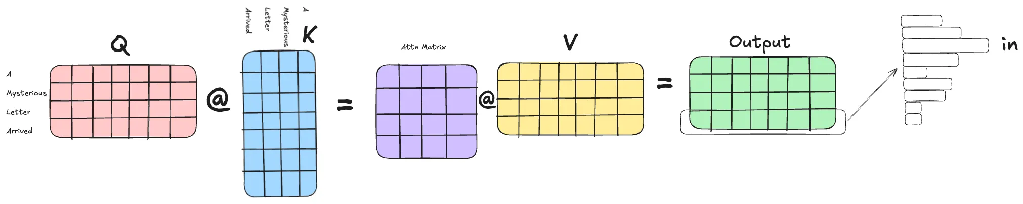
Let’s take a sentence “A mysterious letter arrived”, after passing through a bunch of transformer layers we get the output matrix which in the image above is of 4 x 7 dimension and to predict the next token we choose the embeddings corresponding to the last token “arrived” and project it to vocab size using a mlp layer and we get probabilities over which token to pick next and we sample over that probabilities to pick the next token, in this case it’s “in”. Now let’s generate the next token.

Step 2

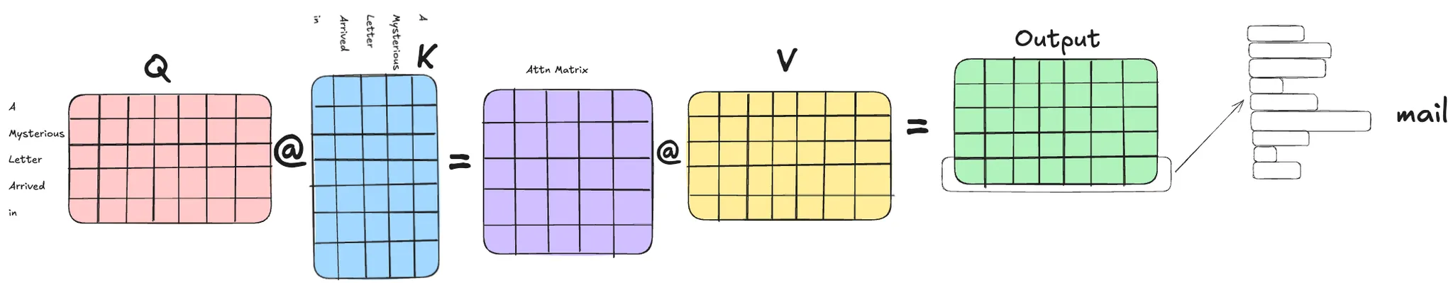
To generate the next token, what we do is simply append the token for “in” to the input tokens (”A mysterious letter arrived”) and now the current input is (”A mysterious letter arrived in”) and given this input, the model will predict the next token. Now you can see the Q, K and V matrices have one additional row/column corresponding to the new token “in” and attention matrix is of size 5x5 now, instead earlier it was 4x4. Then for the next prediction we pick the output embedding corresponding to the token “in” and get probabilities over next token and sample the next token, which in this case is “mail”. Crucially, notice that in this second step, we recalculated the Q, K, and V values for the first four tokens ("A mysterious letter arrived") even though those values have not changed since Step 1. This is the massive, repeated computation we will optimize later.

Okay, let's write some code for this simple generation loop in mlx and later observe the savings.

Everything I’ve explained above about obtaining logits from the model, using the latest token, obtaining probabilities over the next token and sampling the next token (greedy sampling in my case), is implemented here.

KV Cache Optimization

Now let’s take a closer look. Does the fact that we use only the embeddings of the latest token to produce a new token give us some clues about unwanted computation?

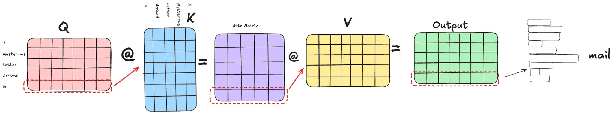
Observation 1: If we backtrack and observe the embeddings that we want from the output matrix, which is the embeddings corresponding to the latest token “in” is obtained, we can see that it is obtained from the last row of attn matrix, which is itself obtained from last row of the query matrix, that means we’re essentially wastefully computing the full Q matrix for tokens (”A mysterious letter arrived”) which is clearly unnecessary.

Observation 2: Another observation is that if you compare the first two figures for generating token “in” and token “main”, we if focus on K and V matrices, we are calculating K and V matrices for (”A”, “mysterious”, “letter”, “arrived”) for generating token “in” and (”A”, “mysterious”, “letter”, “arrived”, “in”) for generating the next token “mail”, and you can see that for every new token generation we are wastefully computing K and V matrices from the beginning over and over again (in this case for tokens (”A”, “mysterious”, “letter”, “arrived”). Now this is redundant, what if everytime we calculate these K and V values, keep them saved and only generate K and V for the latest token and append that to previously saved K and V to proceed with attention computation.

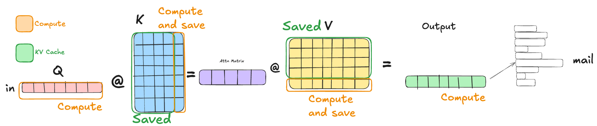
You can see from the diagram above, since we only need the embedding information of the latest token “in” to predict the next token we compute 1.) Q values only for that token, 2.) We compute K and V values for that token and append saved KV value for previous tokens. This way as the context length for the next token generation increases we are not bottlenecked by computation since we’re essentially computing these only one token at a time.

Computationally while calculating Q @ K, we’re reducing from (L x D @ D x L) → (1 x D @ D x L) and at attn_scores @ V we’re reducing from (L x L @ L x D) → (1 x L @ L x D), along with, while computing K, V from inputs, we’re reducing from (L x D’ @ D’ x D) → (1 x D’ @ D’ x D).

Implementing KV Cache using MLX

This implementation has a naive KV cache implementation, this setup has very minor changes to the model

Prefill and Decode

The other interesting thing at the generation loop using caches is, we can divide the generation phase into two stages. Prefill and Decode.

Once the user provides a prompt which contains n tokens, we can prefill the cache with KV values of these tokens and since we are not restricted with autoregression here, we can process and save KVs for bunch of tokens at once.

Once we prefill the cache for n-1 tokens, we use that last token to start the decoding process where the autoregressive nature kicks in and as each token is passed through the model it gets saved in the cache objects and for next generation, we will only need the latest generated token to generate the next one.

You can observe this prefill and decode stages in the naive_cached_generate function.

Performance

Generation Time Without KV Cache: 0.183353s

Generation Time KV Cache: 0.037206

Speedup: 4.928026138343503x, on M3 Pro Macbook

5x improvement over a very naive implementation is not bad, there are a bunch of other optimizations we can do in caching implementation, the literature goes so deep with variants like QuantizedCache for improving memory, SlidingWindowCache for managing large context sizes, PagedAttention, Cross-Layer KV Sharing, KV Cache Eviction Policies with Multi Query Attention (MQA), Grouped Query Attention (GQA), Sliding Window Attention, Speculative Decoding etc. Let’s keep going!